valfera112, Author at Fera Analytics

The real estate price prediction in Ames, Iowa is a popular competition on Kaggle and provides a great dataset to apply creative feature engineering and advanced regression techniques. In this paper, we analyzed the training and test data sets using uni-variate and bi-variate techniques, handled missing values, dealt with outliers, applied machine learning models and tuned hyper parameters.

Datasets

Competitors are given training and test datasets: Training set has 1460 rows and 81 columns and test has 1459 rows and 80 columns (test set has no target variable). We import our csv files and load the data to Pandas dataframes.

Exploratory Data Analysis (EDA)

Categorical vs Numeric Variables We start by splitting our data that includes 81 variables into 45 categorical features and 36 numerical predictors. This gave us a good introduction to the dataset and allowed us to come up with a logical approach to our data wrangling. We observed that some of our numerical variables would be better represented as categories, as their numerical values were not intended to be interpreted as a magnitude.

Binning

Binning is widely used to create a better linear relationship between the predictors and the target. We choose to use binning for the below predictors. Note that, original (unbinned) predictors must be dropped after binning.

Dummification

Some numerical variables are not continuous and must be regarded as categorical variables.

MSSubClass
OverallQual
OverallCond
BsmtFullBath
BsmtHalfBath
FullBath
HalfBath
BedroomAbvGr
KitchenAbvGr
TotRmsAbvGrd
Fireplaces
GarageCars
YrSold

We cast them to category type together with the newly created binned variables and then dummify them with all other categorical variables.


from_num_to_cat = ['MSSubClass','OverallQual','OverallCond','BsmtFullBath','BsmtHalfBath','FullBath','HalfBath','BedroomAbvGr','KitchenAbvGr','TotRmsAbvGrd','Fireplaces','GarageCars','MoSold_Binned','YearBuilt_Binned','YearRemodAdd_Binned','YrSold','GarageYrBlt_Binned','PoolArea_Binned']

df_concat[from_num_to_cat] = df_concat[from_num_to_cat].apply(lambda x: x.astype('category'))

df_concat_dummified = pd.get_dummies(df_concat, drop_first=True)

Missing Values We continue by detecting missing data and resolving the missing values appropriately.

For many of our variables, missing data indicates that the property does not include such feature. This is the case for features describing pools, alleys, fences, fireplaces, basements, and miscellaneous. For categorical features, we should impute ‘None’ and for numerical variables describing these features, we should impute 0. For missing values due to lack of information, we choose to impute with the median because it is more robust to outliers than imputing with the mean. For features with very few unique values, we can impute with the mode. We were able to successfully account for all missing values and continued with our EDA. Uni-variate Analysis We use histograms to illustrate how symmetric (or asymmetric) our data is. This will give us a sense on what transformations we need to make before doing any modelling. By this point we already suspect that we will be using some multi-linear regression to make our predictions. Regression plots are helpful to see the linear relationship between each predictor and the target.

Outliers

Outlier detection and elimination is a very important before applying any machine learning model on a data set. Even one outlier can alter the model predictions dramatically. Outliers can be detected several ways but the most efficient is to visualize data using scatter plots.

The above scatter plot of GrLivArea to target variable SalePrice shows that there are 2 data points with huge living area but comparably lower SalePrice. We remove those observations so that our predictions are more robust when we input unseen test data, and are not skewed by our outliers.

Feature Engineering and Selection

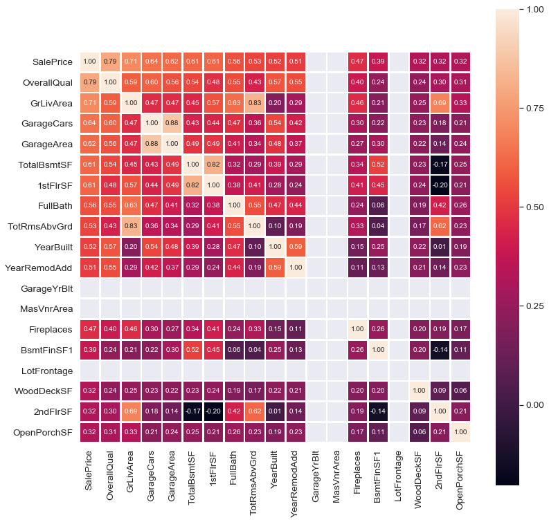
Another important part of EDA is to check for the correlation. The best way to visualize correlation is to use the heatmap.

Some columns in the data set are redundant because they are simply a part of another column. For example; below equations hold so that the added variables provide no value to the models. Dropping them will reduce multicollinearity, too.

BsmtFinSF1 + BsmtFinSF2 + BsmtUnfSF = TotalBsmtSF

1stFlrSF + 2ndFlrSF + LowQualFinSF = GrLivArea

OpenPorchSF + EnclosedPorch + 3SsnPorch + ScreenPorch + WoodDeckSF = TotalPorchSF


df_concat.drop(['BsmtFinSF1', 'BsmtFinSF2', 'BsmtUnfSF'], axis=1, inplace=True)
df_concat.drop(['1stFlrSF','2ndFlrSF','LowQualFinSF'], axis=1, inplace=True)
df_concat.drop(['OpenPorchSF','EnclosedPorch','3SsnPorch','ScreenPorch','WoodDeckSF'], axis=1, inplace=True)

Data Transformations

Log Transform

Taking logarithm of a continuous variable is often used to solve for the skewness. Below figure reveals that target variable SalePrice is highly skewed.

sns.distplot(train['SalePrice']);

# skewness and kurtosis
print("Skewness: %f" % train['SalePrice'].skew())
print("Kurtosis: %f" % train['SalePrice'].kurt())

Observe the skewness and the histogram after we apply log transformation on the target variable.

Modelling

We use Python’s scikit-learn package because it provides all models we need and its object oriented approach makes it easy to fit models.

Preparations

Some preparations are needed before going to the modelling. Since we combine the train and test data sets for east manipulation, we now need to separate them back into train and test. Since test data set must not have target variable, we drop SalePrice_Log even though it consists of all NAs and drop the index.

test = df_concat_dummified.loc[df_concat.SalePrice_Log.isnull(),]
train = df_concat_dummified.loc[~df_concat.SalePrice_Log.isnull(),]
test.drop('SalePrice_Log', inplace=True, axis=1)
test.reset_index(drop=True, inplace=True)

Furthermore, we initialize a Pandas data frame for submitting the predictions with the Id column from the test data set. To fit the models, we specify X (predictors) and Y (target). Be mindful that X must not have Id and SalePrice_Log so that we drop them. There is no need for Id column for test data set as well so we drop Id from test, too.

submission = pd.DataFrame()
submission['Id'] = test.Id

Y=train['SalePrice_Log']
X=train.loc[:, ~train.columns.isin(['Id','SalePrice_Log'])]
test2=test.loc[:, ~test.columns.isin(['Id'])]

Last step before modelling is to check for dimensions of train and test and any nulls, positive or negative infinity.

print(X.shape)
print(test2.shape)
print(set(X.columns) - set(test2.columns))
print(len(set(X.columns) - set(test2.columns)))
print(set(test2.columns) - set(X.columns))
print(X.isin([np.nan, np.inf, -np.inf]).any(axis=0).any())

Multiple Linear Regression

We only use numerical columns as predictors for multiple linear regression. First, we simply add all numerical columns to the regression model and check whether the coefficients are significant or not. However, we need to split the training data as train and test to figure out the train and test errors after fitting. We employ a split of 30% test size and 70% train size.

X_train, X_test, y_train, y_test = train_test_split(X, Y, test_size=0.3, random_state=42)

OLS Regression Results                            
==============================================================================
Dep. Variable:          SalePrice_Log   R-squared:                       0.902
Model:                            OLS   Adj. R-squared:                  0.900
Method:                 Least Squares   F-statistic:                     366.4
Date:                Mon, 10 Jun 2019   Prob (F-statistic):               0.00
Time:                        08:49:30   Log-Likelihood:                 670.21
No. Observations:                1020   AIC:                            -1288.
Df Residuals:                     994   BIC:                            -1160.
Df Model:                          25                                         
Covariance Type:            nonrobust                                         
================================================================================
                   coef    std err          t      P>|t|      [0.025      0.975]
--------------------------------------------------------------------------------
const           14.3594      6.164      2.330      0.020       2.264      26.455
BedroomAbvGr    -0.0268      0.008     -3.566      0.000      -0.042      -0.012
BsmtFullBath     0.0732      0.009      8.362      0.000       0.056       0.090
BsmtHalfBath     0.0068      0.017      0.398      0.691      -0.027       0.040
Fireplaces       0.0437      0.007      5.896      0.000       0.029       0.058
FullBath         0.0198      0.012      1.637      0.102      -0.004       0.043
GarageArea    9.434e-05   4.31e-05      2.187      0.029    9.67e-06       0.000
GarageCars       0.0318      0.014      2.340      0.019       0.005       0.058
GarageYrBlt   3.075e-05   1.18e-05      2.607      0.009     7.6e-06    5.39e-05
GrLivArea        0.0003   2.03e-05     12.860      0.000       0.000       0.000
HalfBath         0.0210      0.010      2.030      0.043       0.001       0.041
KitchenAbvGr    -0.0648      0.023     -2.815      0.005      -0.110      -0.020
LotArea       1.987e-06   3.92e-07      5.073      0.000    1.22e-06    2.76e-06
LotFrontage      0.0004      0.000      1.890      0.059   -1.44e-05       0.001
MSSubClass      -0.0004      0.000     -3.422      0.001      -0.001      -0.000
MasVnrArea    1.588e-05   2.78e-05      0.570      0.568   -3.87e-05    7.05e-05
MiscVal      -2.386e-05   1.24e-05     -1.925      0.055   -4.82e-05    4.65e-07
MoSold           0.0011      0.002      0.701      0.484      -0.002       0.004
OverallCond      0.0479      0.004     10.842      0.000       0.039       0.057
OverallQual      0.0677      0.005     13.115      0.000       0.058       0.078
PoolArea      3.677e-05      0.000      0.291      0.771      -0.000       0.000
TotRmsAbvGrd     0.0155      0.005      2.849      0.004       0.005       0.026
TotalBsmtSF      0.0001   1.43e-05      9.789      0.000       0.000       0.000
YearBuilt        0.0029      0.000     11.700      0.000       0.002       0.003
YearRemodAdd     0.0011      0.000      3.593      0.000       0.000       0.002
YrSold          -0.0058      0.003     -1.873      0.061      -0.012       0.000

Having all numerical variables included as predictors, we have an adjusted R2 of .9 and test error of .885.

Train error is: 0.902
Test error is: 0.885

To determine the coefficients with 0 lying within confidence interval, we issue the command below:

table[table['p value']>=0.05][['name','coef','p value']]

name	coef	p value
3	BsmtHalfBath	0.006800	0.691
5	FullBath	0.019800	0.102
13	LotFrontage	0.000400	0.059
15	MasVnrArea	0.000016	0.568
16	MiscVal	-0.000024	0.055
17	MoSold	0.001100	0.484
20	PoolArea	0.000037	0.771
25	YrSold	-0.005800	0.061

After refitting the multiple linear regression model using only the significan coefficients, we find that train error is a bit lower but the test error is a bit higher. It is not much improvement as we expected but still we decide to go on with the reduced model.

print('Train error: %.5f' %mlr.score(X_train_significants, y_train))
print('Test error: %.5f' %mlr.score(X_test_significants, y_test))

Train error: 0.89998
Test error: 0.88699

Ridge

Ridge is a regularized model so that it needs to be tuned for hyper parameters. Penalty term (alpha) is a hyper parameter to tune. and if it is large, model has less variance but it may suffer from high bias. We use cross-validation to find the best alpha considering different combinations of normalization and intercept parameters.

Alpha range = linspace(0.01, 5, 200)
Cross-validation folds = [3, 5, 10, sqrt_n]
Normalization = [False, True]
Intercept = [False, True]

200 alpha X 4 CV X 2 Norm X 2 Intercept = 3200 config Below table shows the training and test R2 values, mean squared error and average cross-validation error for each combination of cross-validation folds, normalization and intercept. Values for CV are experimentally proven that they are the best candidates to find the optimum for the variance-bias tradeoff. P.S. sqrt_n is the square root of number of observations. The strategy here is to choose the alpha giving the maximum R2 for the test data set. Hence, we choose; alpha=0.41, CV=10, normalization=TRUE, intercept=FALSE

CV	Norm Type	Intercept Type	Alpha	R2 Training	R2 Test	MSE	Avg. CV Score
CV_3	TRUE	TRUE	0.34	0.94307	0.86306	0.01809	0.90146
CV_3	TRUE	FALSE	0.39	0.94784	0.89691	0.02134	0.85406
CV_3	FALSE	TRUE	5	0.94958	0.86306	0.01611	0.90035
CV_3	FALSE	FALSE	0.39	0.94784	0.88388	0.02134	0.85406
CV_5	TRUE	TRUE	0.21	0.94769	0.86303	0.01805	0.90681
CV_5	TRUE	FALSE	0.29	0.95005	0.89718	0.02135	0.86948
CV_5	FALSE	TRUE	4.17	0.9507	0.86303	0.01607	0.91139
CV_5	FALSE	FALSE	0.29	0.95005	0.88419	0.02135	0.86948
CV_10	TRUE	TRUE	0.16	0.94968	0.86299	0.01808	0.90625
CV_10	TRUE	FALSE	0.41	0.94736	0.89738	0.02135	0.86789
CV_10	FALSE	TRUE	3.27	0.95204	0.86299	0.01604	0.91051
CV_10	FALSE	FALSE	0.41	0.94736	0.88408	0.02135	0.86789
CV_31	TRUE	TRUE	0.16	0.94968	0.86299	0.01808	0.90048
CV_31	TRUE	FALSE	0.41	0.94736	0.89736	0.02135	0.8682
CV_31	FALSE	TRUE	3.5	0.95169	0.86299	0.01604	0.90696
CV_31	FALSE	FALSE	0.41	0.94736	0.88408	0.02135	0.8682

Lasso

Lasso is another regularized model. Only difference from Ridge is Lasso has L1 penalty such that when alpha is large enough, coefficients of the predictors are pushed to become 0. That is why Lasso allows for predictor selection. We use the same approach as we did for Ridge and the best alpha we get is: alpha=0.16, CV=5, normalization=TRUE, intercept=FALSE

ElasticNet

ElasticNet is a combination of Ridge and Lasso and introduces an additional hyper parameter to tune. Rho specifies how much Ridge (or Lasso) one intend to use in the model.

Alpha range = np.linspace(0.1, 10, 100)
Rho range = np.linspace(0.01, 1, 100)
Cross-validation folds = [3, 5, 10, sqrt_n]
Normalization = [False, True]
Intercept = [False, True]
P.S. Set max_iter = 10,000 to solve convergence problem

100 Alpha X 100 Rho X 4 CV X 2 Norm X 2 Inter = 160K config Best hyper parameters we get: alpha=0.01, rho=0.01, CV=10, normalization=TRUE, intercept=FALSE

Random Forest

Random forest does not need categorical columns to be dummified so that we omit them in this model. It also has a lot of parameters to tune. Below are the ones we find important:

Randomly select samples
bootstrap = [True, False]
Max. # of levels in tree
max_depth = [10, 20, 30, 40, 50, 60, 70, 80, 90, 100, 110, None]
Max. # of features to consider at each split
max_features = [‘auto’, ‘sqrt’]
Min. # of samples required to split node
min_samples_leaf = [1, 2, 4]
Min. # of samples required to split node
min_samples_split = [2, 5, 10]
# of Trees
n_estimators = [200, 400, 600, 800, 1000, 1200, 1400, 1600, 1800, 2000]

2 BS X 12 Levels X 2 Feat X 3 Leafs X 3 Samples X 10 Estimators = 4320 config Using grid search to find the best parameters, we end up with the below summary table:

CV	R2 Training	R2 Test	Avg CV Score	MSE
CV_3	0.94598	0.7622	0.723	0.03715
CV_5	0.946	0.76201	0.74271	0.03718
CV_10	0.94571	0.76276	0.72345	0.03706
CV_31	0.94582	0.76377	0.70945	0.03691

Since scores are very close to each other, we employ CV=5 and CV=31 which provides best average CV score and best test R2 score, respectively.

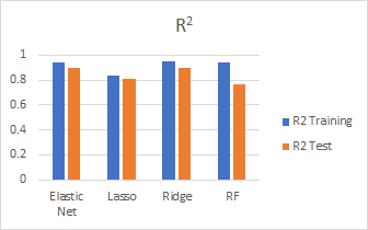
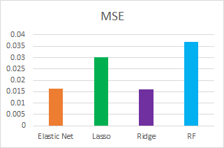
Model Comparison

We compare the models we fit using different metrics such as test R2, MSE and CV scores:

Model Results

Here are the best predictions results submitted for each model:

SubmissionNo	Model	Parameters	Score
16	Ridge	CV=10, Norm=T, Int=F, alpha=0.41	0.12757
19	ElasticNet	CV=10, Norm=T, Int=F, alpha=0.01, rho=0.01	0.12866
11	Lasso	CV=5, Norm=T, Int=F, alpha=0.01	0.12946
15	RandomForest	CV=5, trees=1000	0.14313

In general, Ridge performed the best and random forest performed the worst. Our best score is 0.12757 with Ridge.

Future Work

We believe there may be some improvements both in the feature engineering and modelling parts of the project. If we are given more time, we think that new features can be added to the model and then we can check for any improvement happen in terms of test error. Another improvement point is that we employ XGBoost but do not have enough time to find the best parameters. We think, XGBoost can give better results when tuned properly. Lastly, ensembling can be applied to the trained models, so that a combination of each can be implemented as a final model. Ensembling may allow for better predictions since each model learns a different part of the data.

Introduction:

Forbes Global 2000 ranks the largest companies in the world and provides financial metrics including market capitalization, assets, profits, and sales. I used Selenium and chromedriver to web scrape the list, along with each company’s page. This entailed making the program first scroll to the bottom of the page to load the content and then scroll back to the top to start scrubbing the data. I also ran a separate web scraper that would scrape the data I needed and click to the next page for all 2000 companies. I imported the data into comma delimited files, which yielded two dataframes that I merged to begin my analysis.

Overview

After some cleaning of the data, I ended up with each company’s rank, country, year founded, chairman, industry, assets, sales, profits, market capitalization, and number of employees. The data included companies from 60 countries and collectively accounted for $39.1 trillion in sales, $3.2 trillion in profit, $189 trillion in assets, and $56.8 trillion in market value.

I wanted to illustrate the distribution of these companies across the countries around the world, find the most prevalent industries, and see how the industries around the world differ from those in the United States. I also wanted to go a bit deeper and try to discover some underlying pattern in the data, including any relationship between sales, profit, assets, and market value. My goal was to see if there was a difference in these patterns among the mega-large companies and the rest of the list.

Top 20 Countries on the list

This shows that the overwhelming majority of companies are based in the US, followed by Japan and China. Nearly half of the list comes from the rest of the world.

Industries: Global vs US

Regional banking is the leading industry across the globe. However, inspection of US industries yields some interesting results. We see that Oil and Gas Operations, Investment Services, Electric Utilities, and Real Estate are all more prevalent than Regional Banking in the US.

Relationships Between Assets, Sales, Market Capitalization, and Profit

I created scatter plots with a line of best fit to illustrate the relationship between the different variables in the data that I scraped. There was a positive correlation between assets and sales, assets and market capitalization, assets and profit, market capitalization and profit, market capitalization and sales.

Interestingly, there does not seem to be a relationship between assets and sales, assets and market capitalization, assets and profit for those companies falling lower on the Forbes List.

Correlation Heatmap

I created a heatmap of the correlation matrix to further illustrate this trend in the data. We can see the strongest correlation is between market cap and profits, and this is especially true for the highest ranking companies on the list.

Interestingly, there is a negative correlation between market cap and assets for those companies falling in the middle of the list.

Author: valfera112

Real Estate Price Predictions